Formulation

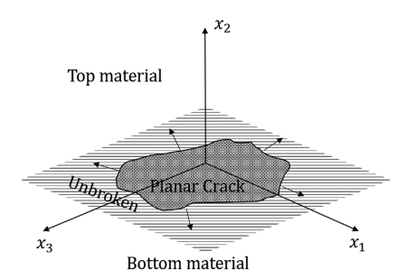
Fig. 1 A three-dimensional rupture propagation in a plane.

Consider a 3D fracture plane as given shown in Fig. 1. The elastodynamic equations at the interface between two dissimilar elastic half-spaces is given as follows (Kostrov, 1966; Gupta and Ranjith, 2024):

\[A_{ij}(\tau_{i}(x_1,x_3,t)-\tau_{i}^0(x_1,x_3,t))+ \dot{\delta}_i(x_1,x_3,t) = f_i (x_1,x_3,t)\]

where, \(x_i\) is a Cartesian coordinate system, with \(x_1-x_3\) plane being the plane of interface and time \(t\). \(\left[A_{ij} \right]\) is a diagonal matrix with \(A_{11} = A_{33} = \frac{c_s^+}{\mu^+}\), \(A_{22} = \frac{c_d^+}{\lambda^+ + 2 \mu^+}+\frac{c_d^-}{\lambda^- + 2 \mu^-}\). \(\tau_{i}\)’s are the traction components at the interface with stresses at the interface being \(\tau_{i}(x_1,x_3,t)= \sigma_{i2}(x_1,x_2^{\pm},x_3,t)\). \(\dot{\delta}_i\) is the rate of discontinuity at the interface with \(\delta_i\) given in terms of displacements \(u_i\) of the two half-spaces as \(\delta_i = u_i^+ - u_i^-\). The superscripts “\(\pm\)” refer to field quantities corresponding to the top and lower half-space, respectively. \(\lambda\) and \(\mu\) are the Lame's parameters. The shear and dilatational wave speeds are given by \(c_s = \sqrt{\mu/\rho}\) and \(c_d = \sqrt{(\lambda +2\mu )/\rho}\), respectively, with \(\rho\) being the density of the elastic half-space. The functionals \(f_i\)’s involve the spatio-temporal convolutions of traction components at the interface.

Spectral BIEM

In spectral BIEM, the field quantities traction and slip (displacement discontinuities) at the interface are taken in spectral form as:

\[\begin{split}\begin{Bmatrix} \tau_j(x_1,x_3,t) \\ \delta_j(x_1,x_3,t) \\ \end{Bmatrix} = \begin{Bmatrix} T_j(t;k,m) \\ D_j(t;k,m) \\ \end{Bmatrix} e^{i(kx_1+mx_3)},\end{split}\]

where \(k\) and \(m\) are wave numbers in \(x_1\) - and \(x_3\) - directions. Let, \(q = (k , m)\) is a two-dimensional wave vector, with a magnitude \(q=\sqrt{k^2 + m^2}\).

We get the 3D Spectral BIEM relations (see. Eq. 19 in Gupta and Ranjith, 2024) at the interface of two dissimilar half-spaces as:

\[\begin{split}\begin{bmatrix} \frac{c_s^+}{\mu^+} \eta T_1 \left( t; k, m \right) + \frac{\partial D_1\left(t; k, m \right)}{\partial t} \\ \frac{c_s^+}{\mu^+} \xi T_2 \left( t; k, m \right) + \frac{\partial D_2\left(t; k, m \right)}{\partial t} \\ \frac{c_s^+}{\mu^+} \eta T_3 \left( t; k, m \right) + \frac{\partial D_3\left(t; k, m \right)}{\partial t} \end{bmatrix} = \begin{bmatrix} F_1 \left( t; k, m \right) \\ F_2 \left( t; k, m \right) \\ F_3 \left( t; k, m \right) \end{bmatrix}\end{split}\]

where, \(\eta = \left( 1+ \frac{c_s^-}{c_s^+}\frac{\mu^+}{\mu^-}\right)\) and \(\xi = \left( \frac{c_s^+}{c_d^-} + \frac{c_s^-}{c_s^+}\frac{\mu^+}{\mu^-}\frac{c_s^-}{c_d^-}\right)\), and the convolution terms are given by

\[\begin{split}\begin{Bmatrix} F_1 \left( t; k, m \right) \\ F_2 \left( t; k, m \right) \\ F_3 \left( t; k, m \right) \end{Bmatrix} = \int_0^t \begin{bmatrix} C_{11} \left( t'; q \right) & C_{12} \left( t'; q \right) & C_{13} \left( t'; q \right) \\ C_{21} \left( t'; q \right) & C_{22} \left( t'; q \right) & C_{23} \left( t'; q \right) \\ C_{31} \left( t'; q \right) & C_{32} \left( t'; q \right) & C_{33} \left( t'; q \right) \end{bmatrix} \begin{bmatrix} T_1 \left( t - t'; k, m \right) \\ T_2 \left( t - t'; k, m \right) \\ T_3 \left( t - t'; k, m \right) \end{bmatrix} dt'\end{split}\]

In the above equation, we have five independent convolution kernels which can be expressed as

\[\begin{split}C_{11} (t; q) = \frac{1}{q^2} [k^2 (M_{11}^+ + M_{11}^-) + m^2 (M_{33}^+ + M_{33}^-)] \\ C_{22}(t; q) = M_{22}^+ + M_{22}^- \\ C_{33}(t; q) = \frac{1}{q^2} [m^2 (M_{11}^+ + M_{11}^-) + k^2 (M_{33}^+ + M_{33}^-)] \\ C_{12}(t; q) = \frac{k}{m} C_{22}(t; q) = -\frac{m}{k} C_{33}(t; q) = -C_{21}(t; q) = \frac{k}{q^2} [M_{12}^+ - M_{12}^-] \\ C_{13}(t; q) = C_{31}(t; q) = \frac{km}{q^2} [ (M_{11}^+ + M_{11}^-) - (M_{33}^+ + M_{33}^-) ]\end{split}\]

All above convolution kernels \(\left( C_{ij}(t; q) \right)\) can be expressed in closed form. The convolution kernels \(M_{11}(t; q), M_{12}(t; q), M_{22}(t; q)\) and \(M_{33}(t; q)\) can be written as in the Appendix of Gupta and Ranjith, 2024):

\[\begin{split}\begin{split} M_{11}(t; q) =& c_s \frac{c_s}{\mu} |q| \Bigg\lbrace - \int_0^1 \frac{g(y) - g(y_R)}{y - y_R} y \sin(|q| c_s t) \, dy \\ & + g(y_R) \Bigg[y_R \sin(|q| c_R t) \int_{|q|c_s t - |q|c_R t}^{|q|c_s t + |q|c_R t} \cos \theta \, d\theta - y_R \cos(|q|c_R t) \int_{-|q|c_R t}^{|q|c_R t} \sin\theta \, d\theta \Bigg] \\ & + g(y_R) \frac{\cos(|q|c_s t) - 1}{|q| c_s t} \frac{2}{\pi} \int_1^a \frac{4(1-y^2)\sqrt{1-y^2/a^2}}{(y^2 - y_R^2)(y^2-y_1^2)(y^2-y_2^2)} y \sin(|q|c_s t) \, dy \Bigg\rbrace \end{split}\end{split}\]

\[\begin{split}\begin{split} M_{22}(t; q) =& c_s \frac{c_s}{\mu} |q| \Bigg\lbrace - \int_0^1 \frac{f(y) - f(y_R)}{y - y_R} y \sin(|q| c_s t) \, dy \\ & + f(y_R) \Bigg[ y_R \sin(|q| c_R t) \int_{|q|c_s t - |q|c_R t}^{|q|c_s t + |q|c_R t} \cos \theta \, d\theta - y_R \cos(|q|c_R t) \int_{-|q|c_R t}^{|q|c_R t} \sin\theta \, d\theta \Bigg] \\ & + f(y_R) \frac{\cos(|q|c_s t) - 1}{|q| c_s t} \frac{2}{\pi} \int_1^a \frac{(2-y^2)\sqrt{1-y^2/a^2}}{(y^2 - y_R^2)(y^2-y_1^2)(y^2-y_2^2)} y \sin(|q|c_s t) \, dy \Bigg\rbrace \end{split}\end{split}\]

\[\begin{split}\begin{split} M_{12}(t; q) =& -iq c_s \frac{c_s}{\mu} \frac{2}{\pi} \int_1^a \Bigg[ \frac{2y\sqrt{2 - 1 - y^2 / a^2}(2-y^2)}{(y_R^2 - y^2)(y_1^2 - y^2)(y_2^2 - y^2)} \cos(y|q|c_s t) \\ & + \frac{-8y_R^2/a^2 + 8/a^2 - y_R^4 + 4 + 6y_R^2 + 2\sqrt{1-y_R^2/a^2}(2-y_R^2)}{(y_1^2 - y_R^2)(y_2^2 - y_R^2)} \cos(|q|c_R t) \Bigg] \end{split}\end{split}\]

\[M_{33}(t; q) = c_s \frac{c_s}{\mu} J_1(|q|c_s t)\]

with

\[g(y) = \frac{2}{\pi} \frac{4\,(1-y^2)\, \sqrt{1-y^2/a^2} + (2-y^2)^2 \sqrt{1-y^2}}{(y + y_R) \, (y^2 - y_1^2)\, (y^2 - y_2^2)}\]

\[f(y) = \frac{2}{\pi} \frac{4\,(1-y^2/a^2)\, \sqrt{1-y^2} + (2-y^2)^2 \sqrt{1-y^2/a^2}}{(y + y_R) \, (y^2 - y_1^2)\, (y^2 - y_2^2)}\]

where \(s = p / \|q\| c_s, a = c_d / c_s\), and \(y_R = c_R / c_s\). \(c_R\) is the Rayleigh wave speed.

Interface Law

We have incorporated the classical linear friction slip-weakening law in the code. The frictional coefficients are vectorized over the fault plane so that one can analyze the effect of local heterogeneities. One can look into the main.cuf in the ./src directory to add more frcitional law as an when necessary.

Linear Slip-Weakening law

The linear slip-weakening friction law is as follows:

\[\begin{split}\tau_2^{*}(\delta) = \tau_2 \begin{cases} \mu_s -(\mu_s - \mu_r) \frac{\delta}{\delta_{c}}, & \text{if $\delta < \delta_c$}\\ \mu_r, & \text{otherwise} \end{cases}\end{split}\]

where, \(\tau_2^{*}\) is the effective shear strength of fault plane, \(\delta=\sqrt{(\delta_1^2 + \delta_3^2)}\) is the effective slip, and \(\delta_{c}\) is the critical slip-weakening distance. \(\mu_s\) and \(\mu_r\) are the static and residual frictional coefficients, respectively.